Univariate models

Univariate Assignment

Read in tree data

# read in data directly from website: 
# red maple dataset
maple <- read.csv('https://raw.githubusercontent.com/dmcglinn/quant_methods/gh-pages/data/maple.csv',  
                  stringsAsFactors = TRUE)
# Frasier fir dataset
fir <- read.csv('https://raw.githubusercontent.com/dmcglinn/quant_methods/gh-pages/data/fir.csv',
                stringsAsFactors = TRUE)

Examine this dataset and see how the data is structured, see function str

The contents of the metadata file (./data/tree_metadata.txt) is provided below:

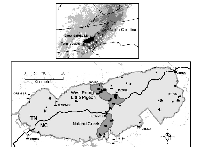
The dataset includes tree abundances from a subset of a vegetation database of Great Smoky Mountains National Park (TN, NC).

• cover: local abundance measured as estimated horizontal cover (ie, relative area of shadow if sun is directly above) classes 1-10 are: 1=trace, 2=0-1%, 3=1-2%, 4=2-5%, 5=5-10%, 6=10-25%, 7=25-50%, 8=50-75%, 9=75-95%, 10=95-100%
• elev: elevation in meters from a digital elevation model (10 m res)
• tci: topographic convergence index, or site “water potential”; measured as the upslope contributing area divided by the tangent of the slope angle (Beven and Kirkby 1979)
• streamdist: distance of plot from the nearest permanent stream (meters)
• disturb: plot disturbance history (from a Park report); CORPLOG=corporate logging; SETTLE=concentrated settlement, VIRGIN=”high in virgin attributes”, LT-SEL=light or selective logging
• beers: transformed slope aspect (‘heat load index’); 0 is SW (hottest), 2 is NE (coolest)

Above shows a map of the regional and local location of the elevational transects included in the dataset (from Fridley 2009).

1. Carry out an exploratory analysis using the two tree datasets. Metadata for the tree study can be found here. Specifically, I would like you to visually examine how the explanatory variables relate to tree cover for a habitat generalist Acer rubrum (Red maple) and a habitat specialist Abies fraseri (Frasier fir).

After carrying out a visual examination of the correlations with tree cover go ahead and build linear multiple regression models and interpret them. This this dataset includes both continuous and discrete (i.e., disturb) explanatory variables so we will use both the functions summary and car::Anova(..., type = 3) to interpret the model. For example, your code will likely look something like:

#install.packages('car') # if you have not installed before
library(car)             # load the library
# build the linear model
my_mod <- lm(cover ~ elev + tci + ... , data = maple)
# where ... represents all of the variables you decide to include in your model
# the function summary() provides a lot of useful information
summary(my_mod)
# to look at the effect of the discrete variable more directly try
Anova(my_mod, type=3)    # example of a type 3 anova

This will estimate partial effect sizes, variance explained, and p-values for each explanatory variable included in the model.

Compare the p-values you observe using the function Anova to those generated using summary.

For each species address the following additional questions:

• what patterns did you notice in your visual examination of the data?
• how well does the exploratory model appear to explain cover?
• which explanatory variables does your model indicate are the most important?
• are these the same variables that your visual examination uncovered?
• do model diagnostics indicate any problems with violations of OLS assumptions?
• are you able to explain variance in one species better than another, why might this be the case (statically or ecologically)?

2. You may have noticed that the variable cover is defined as positive integers between 1 and 10. and is therefore better treated as a discrete rather than continuous variable. Re-examine your solutions to the question above but from the perspective of a General Linear Model (GLM) with a Poisson error term (rather than a Gaussian one as in OLS). The Poisson distribution generates integers 0 to positive infinity so this may provide a good first approximation. Your new model calls will look as follows:

acer_poi = glm(cover ~ tci + elev + ... , data = my_data, 
           family='poisson')

For assessing the degree of variation explained you can use a pseudo-R-squared statistic (note this is just one of many possible)

pseudo_r2 = function(glm_mod) {
                1 -  glm_mod$deviance / glm_mod$null.deviance
            }

Compare your qualitative assessment of which variables were most important in each model. Does it appear that changing the error distribution changed the results much? In what ways?

3. Provide a plain English summary (i.e., no statistics) of what you have found and what conclusions we can take away from your analysis?

4. (optional) Examine the behavior of the function stepAIC() using the exploratory models developed above. This is a very simple and not very robust machine learning stepwise algorithm that uses AIC to select a best model. By default it does a backward selection routine.

5. (optional) Develop a model for the number of species in each site (i.e., unique plotID). This variable will also be discrete so the Poisson may be a good starting approximation. Side note: the Poisson distribution converges asymptotically on the Gaussian distribution as the mean of the distribution increases. Thus Poisson regression does not differ much from traditional OLS when means are large.